This blog post was inspired by Bryan Johnson’s tweet from last March:
This tweet caught my eye: “solve death” and “EBMs” in one sentence. I chuckled, remembering my last encounter with Energy-Based Models (EBMs). Many hours of training, diverging loss curves, and an existential crisis later, I felt much closer to the pits of hell than to the fountain of youth. All jokes aside, let’s dive into the beautiful beasts that are EBMs.
Generative models
Generative models are a class of algorithms designed to learn the underlying distribution of data and generate new samples that resemble the training data. When you are chatting with ChatGPT, there is a generative model generating text back to you. Some popular generative models you may have heard of are Diffusion Models (the stuff that powers Midjourney), VAEs, or GANs.
Each model has advantages and disadvantages, so model selection depends on factors such as data type, computational resources, and training stability. Energy-Based Models (EBMs) represent another class of generative models with their own unique strengths and limitations.
We assume real data follows a complex distribution $p$. We seek model parameters $\theta$ to sample from a model distribution $p_\theta$ that mimics $p$. The aim is to minimize the discrepancy between $p_\theta$ and $p$, allowing us to generate new samples that are indistinguishable from real data.
Introduction to EBMs
EBMs offer a unique approach to generative modeling by framing the problem in terms of an energy function. Unlike other generative models that directly learn to produce data, EBMs learn to assign low energy to likely data configurations and high energy to unlikely ones.
EBMs define an energy function $E_\theta(x)$ parameterized by $\theta$ (for example, a neural network), which maps each possible data configuration $x$ to a scalar energy value. The probability of a data point is then defined as:
\[p_\theta(x) = \frac{\exp(-E_\theta(x))}{Z(\theta)}\]where $Z(\theta) = \int \exp(-E_\theta(x)) dx$ is the normalizing constant.
While this may sound overwhelming, all we have introduced so far is a way to assign non-negative values to data points $\exp(-E_\theta(x))$ and then normalize over the data domain to get a probability distribution. A bit like how you’d normalize a histogram of discrete data points to get a probability mass function.
Sampling EBMs
It’s good to understand how to sample data from EBMs as it is a prerequisite for some of the training methods. One nice property of EBMs is that the gradient:
\[-\nabla_x E_\theta(x)\]points in the same direction as $\nabla_x \log p_\theta(x)$. To demonstrate this, let’s recall the definition EBMs from the introduction:
\[p_\theta(x) = \frac{\exp(-E_\theta(x))}{Z(\theta)}\]Then, taking the logarithm of both sides:
\[\log p_\theta(x) = -E_\theta(x) - \log Z(\theta)\]Now, if we take the gradient with respect to $x$:
\[\nabla_x \log p_\theta(x) = -\nabla_x E_\theta(x)\]The negative gradient of the energy function $-\nabla_x E_\theta(x)$ indicates the direction in which the energy decreases most rapidly. Since lower energy corresponds to higher probability in an EBM, following this negative gradient leads us towards regions of higher probability. If $p_\theta(x)$ approximates $p(x)$ well, we can generate samples that faithfully represent the true data distribution by following this gradient.
This insight leads us to Langevin dynamics, a powerful method for sampling from EBMs. Langevin dynamics combines gradient information with random noise to explore the probability landscape defined by the EBM. The basic Langevin dynamics algorithm is as follows:
- Step 1: Start with an initial point $x_0$, often chosen randomly.
- Step 2: For $t = 0$ to $T$, iterate:
where $z_t \sim \mathcal{N}(0, I)$ is standard Gaussian noise, and $\epsilon$ is a small step size.
This update rule has two key components:
- The gradient term $-\frac{\epsilon}{2} \nabla_x E_\theta(x_{t-1})$ guides the sample towards regions of lower energy (higher probability).
- The noise term $\sqrt{\epsilon} z_t$ allows for exploration of the probability space, helping to escape local minima and sample from the full distribution.
Here is a visualization of how Langevin sampling looks in a simple 2D case (relevant code):
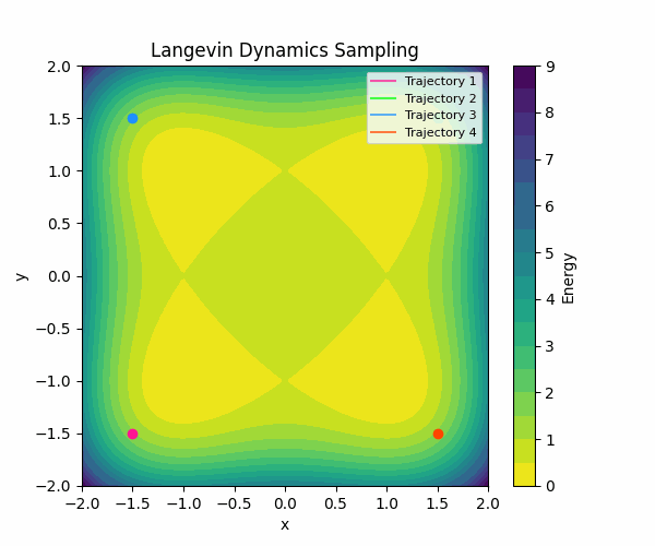
In the visualization above, we start from four different initialization points, and run Langevin sampling in a simple energy landscape with four minima. For more in-depth information about sampling, check out this great blog post by Roy Friedman.
Training EBMs
Unlike classification or regression where we directly get the target values, generative modeling requires us to capture the essence of a data distribution we can’t directly observe. We never actually get $p(x)$, we only have access to samples from this distribution - our training data. So how do we train an EBM to learn an energy function that effectively models this unseen distribution? In this section, we’ll explore a couple of approaches to tackle this problem.
Contrastive divergence
The first approach for training EBMs we explore is rooted in maximum likelihood estimation. In general, MLE aims to maximize the likelihood of the observed data under our model, which is equivalent to minimizing the negative log-likelihood:
\[J(\theta) = -\mathbb{E}_{x \sim p}[\: \log p_\theta(x) \:]\]Expanding this using the definition of $p_θ(x)$ for EBMs:
\[J(\theta) = \mathbb{E}_{x \sim p}[E_\theta(x)] + \log Z(\theta)\]Then, the gradient of this loss with respect to $\theta$ is:
\[\nabla_\theta J(\theta) = \mathbb{E}_{x \sim p}[\nabla_\theta E_\theta(x)] - \mathbb{E}_{x \sim p_\theta}[\nabla_\theta E_\theta(x)]\]This gradient has an intuitive interpretation:
- The first term, $\mathbb{E}_{x \sim p}[\nabla_\theta E_\theta(x)]$, pushes the energy of real data points down.
- The second term, $-\mathbb{E}_{x \sim p_\theta}[\nabla_\theta E_\theta(x)]$, pulls the energy of model samples up.
To get an intuition for what happens, you may find this visualization of a single MLE step helpful:
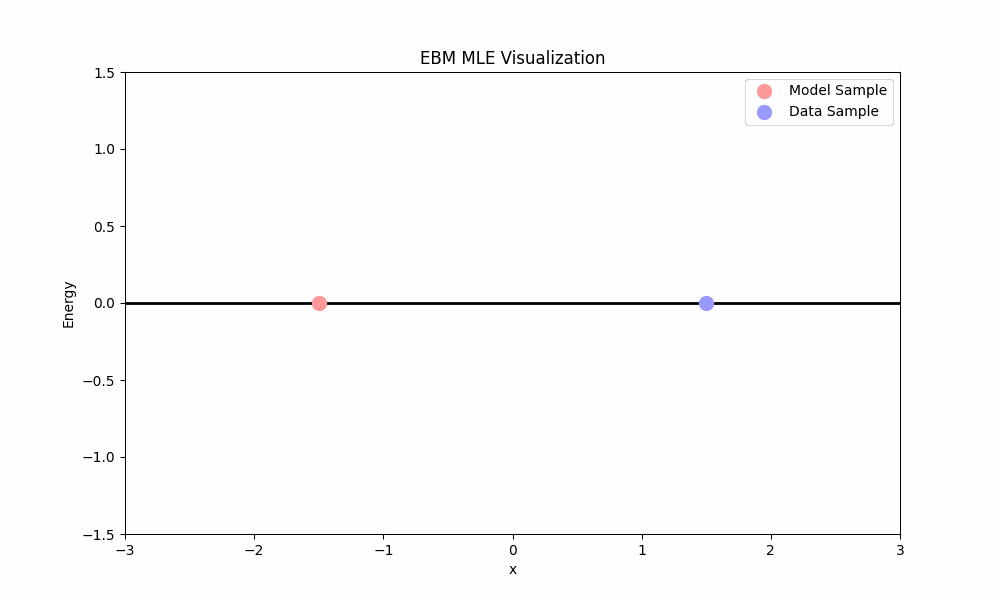
MLE training ideally places low energy in regions with data and high energy elsewhere. Unfortunately, MLE faces a significant practical challenge: computing the expectation over the model requires sampling from $p_\theta$ (e.g., using Langevin dynamics from above), which is computationally expensive.
This is where Contrastive Divergence (CD), introduced by Geoffrey Hinton, comes into play. CD can be viewed as a practical approximation of MLE, designed to make the training process computationally feasible. CD approximates the MLE gradient by replacing the model expectation ($x \sim p_\theta$) with samples obtained by running a few steps of Langevin dynamics starting from data points. These are two simple changes to the Langevin dynamics algorithm we introduced above:
- Step 1: Use data samples to initialize $x_0$. For example, we can sample random data from the batch.
- Step 2: Same as the original, except $T$ is usually in the order of tens of steps.
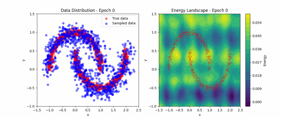
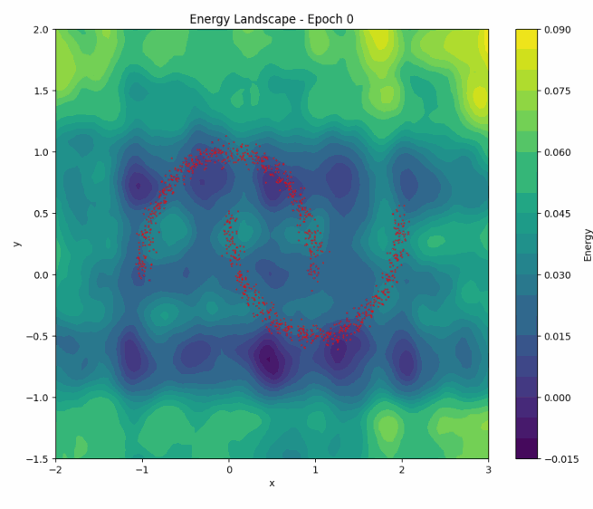
Putting all of this together, we can now fit the simple ‘two moons’ dataset. Below, you can find a visualization of how the EBM samples evolve during contrastive divergence training (left) and the evolution of the full energy landscape (right). Initially, the samples and energy landscape are random, but as training progresses, the model learns to concentrate the low-energy regions around the two crescents of the dataset. You can play around with the code that produced this visualization here.
Score matching
Even though contrastive divergence alleviates some of the difficulties of sampling from the model during training, it still requires running Langevin dynamics for a number of steps. Score matching by Aapo Hyvärinen is an alternative method for training EBMs that completely avoids the need for explicit sampling from the model distribution.
The core idea of score matching is to train the model to match the score function of the data distribution. The score function is defined as the gradient of the log-probability with respect to the input:
\[\psi(x) = \nabla_x \log p(x)\]For an EBM with energy function $E_\theta(x)$, the score function is (see Sampling EBMs for derivation):
\[\psi_\theta(x) = -\nabla_x E_\theta(x) \]The score matching objective is to minimize the expected squared difference between the model’s score and the data score:
\[J(\theta) = \frac{\mathbb{E}_{x \sim p} [\lVert \psi_\theta(x) - \psi(x)\rVert^2]}{2}\]However, we don’t have access to the true data score $\psi(x)$. Fortunately, Hyvärinen showed that this objective can be reformulated into an equivalent form that only requires samples from the data distribution (proof in the Appendix):
\[J(\theta) = \mathbb{E}_{x \sim p} [\frac{1}{2} \lVert \psi_\theta(x) \rVert^2 + \text{tr}(\nabla_x \psi_\theta(x))] + \text{const}\]Returning to the ‘two moons’ example, we can now visualize the evolution of the score function during training. The score function represents the direction and magnitude of the steepest increase in log-probability at each point in the input space. As training progresses, we expect the score function to align with the true data distribution, pointing towards areas of high density.
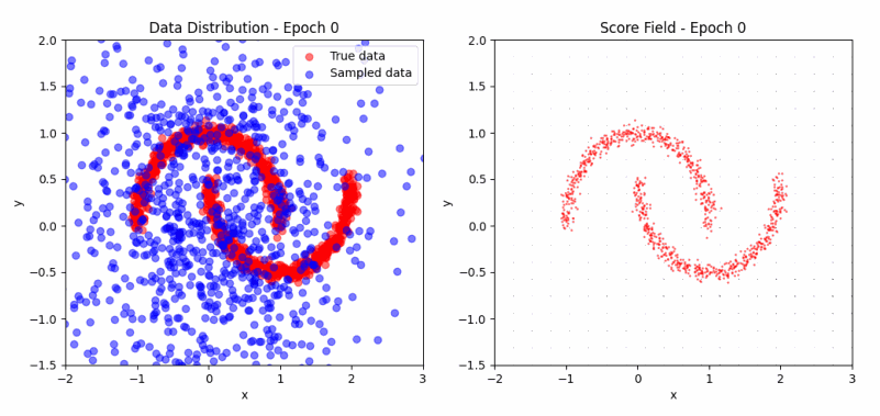
As we can observe in the visualization, the samples (left) evolve from scattered points to the characteristic two-moon shape, while the score field (right) progressively aligns towards areas of high data density. This illustrates how score matching effectively captures the data distribution without explicit sampling. You can experiment with the code here.
Noise contrastive estimation (NCE)
Noise Contrastive Estimation (NCE), introduced by Gutmann and Hyvärinen in 2010, offers another approach to training EBMs. The fundamental concept behind NCE is to train the model to distinguish between samples from the data distribution and samples from a known noise distribution.
In NCE, we introduce a noise distribution $p_n$ (often Gaussian or uniform) alongside our data distribution. We then create a binary classification problem where the model learns to distinguish between data samples (label 1) and noise samples (label 0). The NCE objective is to maximize:
\[J(\theta) = \mathbb{E}_{x \sim p}[\log h(x; \theta)] + \mathbb{E}_{x \sim p_n}[\log (1 - h(x; \theta))]\]where $h(x; \theta)$ is the probability that $x$ comes from the data distribution rather than the noise distribution:
\[h(x; \theta) = \frac{p_\theta(x)}{p_\theta(x) + p_n(x)}\]The NCE loss function has a simple intuitive interpretation:
- Data samples: The first term, $\mathbb{E}_{x \sim p}[\log h(x; \theta)]$, encourages the model to assign high probabilities to real data points.
- Noise samples: The second term, $\mathbb{E}_{x \sim p_n}[\log (1 - h(x; \theta))]$, encourages the model to assign low probabilities to noise samples.
As training progresses, $p_\theta(x)$ should become large for real data points and small for noise samples, shaping the energy landscape to match the true data distribution.
For an EBM, we face a challenge: we want to compute $p_\theta(x)$, but we don’t know the normalization constant $Z(\theta)$. A key insight is that we can treat $\log Z(\theta)$ as a parameter to be learned, avoiding the need to compute it explicitly. We can re-parameterize our model by introducing a new parameter $c = -\log Z(\theta)$. This allows us to write: $p_\theta(x) = \exp(-E_\theta(x) + c)$. Now, instead of learning $\theta$ alone, we learn both $\theta$ and $c$. This approach is viable in NCE because the objective function’s structure prevents trivial solutions where $c$ could grow arbitrarily large, unlike in maximum likelihood estimation.
To illustrate NCE in action, let’s revisit how the energy landscape evolves during training in the ‘two moons’ dataset:
Once again, as training progresses, the model learns to concentrate the low-energy regions around the two crescents of the dataset. You can play with the code here.
EBM problems and practical tips
While the examples above make it look like training EBMs is a piece of cake, the reality is far more challenging. Scaling EBMs to complex, high-dimensional problems often requires a toolbox of sophisticated tricks. Some common issues include:
Poor negatives: You should regularly check the negatives used during training. For NCE, the noise should be “close” to data. For CD, you should make sure sampling produces reasonable examples as training evolves.
Unregularized energy functions: It can be useful to incorporate some L1 / L2 regularization to make the training stable. At the very least, it’s nice if the energy function is bounded so that it can converge. Otherwise, the optimization can just keep increasing the difference between the data and sample energy.
Non-smooth energy functions: When using gradient-based sampling methods like Langevin dynamics with deep neural nets, it can be helpful to implement gradient clipping or forms of spectral regularization. This prevents excessively large updates that can cause the sampling process to diverge.
Slow computation / memory problems: Especially in high-dimensional spaces, sampling becomes a lot more computationally demanding. It is worth considering if the data can be projected to a lower-dimensional space. Alternatively, I’d consider using sampling-free methods (like sliced score matching).
Just learn the score function: This is a fun experience I have with score matching. I found that if you do not need the energy values, it can be easier to learn a function that directly outputs the scores (the gradient of the energy).
Conclusion and further reading
Hope you enjoyed this deep dive into the world of Energy-Based Models!
Remember Bryan Johnson’s tweet that kicked off this whole exploration? Now we have the tools necessary to understand what Extropic proposes. Extropic’s idea seems to be to create physical systems where $E_\theta(x)$ is directly encoded in hardware. Instead of simulating Langevin dynamics on a digital computer, they’re proposing to build circuits where this dynamics occurs naturally. I don’t know enough about hardware to know whether this is viable, but it would be extremely exciting if it works. Better sampling from complex probability distributions could revolutionize how we approach probabilistic AI algorithms, especially those involving EBMs.
For those looking to dive deeper into EBMs and related topics, here are some recommended resources:
- How to Train Your Energy-Based Models - very nice introduction to EBMs following a similar pattern and notation to this blog post by Song et al.
- A Tutorial on Energy-Based Learning - a comprehensive introduction to EBMs by LeCun et al.
- Sliced Score Matching: A Scalable Approach to Density and Score Estimation - more advanced score matching technique by Song et al.
- Generative Modeling by Estimating Gradients of the Data Distribution - another cool score matching extension by Song et al.
- Implicit Generation and Modeling with Energy-Based Models - tricks to get contrastive divergence to scale by Du et al.
- Implicit Behavioral Cloning - EBMs applied to learning policies in robotics by Florence et al.
- Energy-based models for atomic-resolution protein conformations - EBMs applied to proteins by Du et al.
- Collection of awesome EBM papers
Appendix
Proof of score function reformulation
Let’s start with the original score matching objective:
\[J(\theta) = \frac{1}{2} \mathbb{E}_{x \sim p} [\lVert \psi_\theta(x) - \psi(x) \rVert^2]\]Where $\psi_\theta(x) = -\nabla_x E_\theta(x)$ is the model’s score function and $\psi(x) = \nabla_x \log p(x)$ is the true data score function.
We’ll prove that this is equivalent to:
\[J(\theta) = \mathbb{E}_{x \sim p} [\frac{1}{2} \lVert \psi_\theta(x) \rVert^2 + \text{tr}(\nabla_x \psi_\theta(x))] + \text{const}\]Step 1: Expand the squared norm in the original objective:
\[J(\theta) = \frac{1}{2} \mathbb{E}_{x \sim p} [\lVert \psi_\theta(x) \rVert^2 - 2\psi_\theta(x)^T\psi(x) + \lVert \psi(x) \rVert^2]\]Step 2: Focus on the middle term:
\[-\mathbb{E}_{x \sim p} [\psi_\theta(x)^T\psi(x)]\]Step 3: Definition of expectation
\[ -\int p(x) \psi_\theta(x)^T\psi(x) dx\]Step 4: Substitute $\psi(x) = \nabla_x \log p(x)$
\[-\int p(x) \psi_\theta(x)^T\nabla_x \log p(x) dx \]Step 5: Log derivative trick (just applying the chain rule to the log probability)
\[-\int \psi_\theta(x)^T\nabla_x p(x) dx\]Step 6: Integration by parts
Recall the general form of integration by parts:
\[\int u \frac{dv}{dx} dx = uv - \int v \frac{du}{dx} dx\]In our case:
\[\begin{align*}u &= \psi_\theta(x)^T \\\frac{dv}{dx} &= \nabla_x p(x)\end{align*}\]Now, we can apply integration by parts:
\[\begin{align} -\int \psi_\theta(x)^T\nabla_x p(x) dx &= -[\psi_\theta(x)^T p(x)]_{-\infty}^{\infty} + \int p(x) \nabla_x \psi_\theta(x)^T dx \\ &= \int p(x) \nabla_x \psi_\theta(x)^T dx \\ &= \mathbb{E}_{x \sim p} [\text{tr}(\nabla_x \psi_\theta(x))] \end{align}\]Note how $[\psi_\theta(x)^T p(x)]_{-\infty}^{\infty}$ vanished. This is a weak regularity assumption made in the original paper.
Step 7: Combining all the terms
\[J(\theta) = \mathbb{E}_{x \sim p} [\frac{1}{2} \lVert \psi_\theta(x) \rVert^2 + \text{tr}(\nabla_x \psi_\theta(x))] + \frac{1}{2}\mathbb{E}_{x \sim p} [\lVert \psi(x) \rVert^2]\]The last term doesn’t depend on $\theta$, so it’s constant with respect to the optimization. This completes the proof.